

I joined Lyft in January of 2024, as a Data Scientist — Decisions, on the Rider Science Core Experience team. My journey at Lyft began with a starter project, which focussed on using the Rider Experience Score (RES) tool to measure long-term effects of various rider experiences at Lyft.
In this blog post, I will discuss my experience at Lyft as a new hire, focusing on this starter project.
What is RES?
Motivation
At Lyft, we aim to deliver seamless and reliable experiences for our riders. To continuously improve the platform, it’s important to understand which rider experiences most impact our riders, and how those experiences influence their decision to continue using Lyft over time (rider retention).
For example, we can imagine a hypothetical scenario where a rider experiences a lower than normal ETA (the estimated request to pickup time). Experiencing lower ETA can potentially be an improved experience for riders, motivating us to make a product change which drives a decrease in ETA. To justify the introduction of this product change, we first want to quantify how low ETA impacts long-term rider retention. Using an A/B test to evaluate the long-term rider retention impact of low ETA may be problematic, since an A/B test typically runs for 2–6 weeks, which may not be a long enough time period to accurately measure long-term effects. In other cases, A/B tests may not be possible, such as when introducing a new feature which is rolled out to all users.
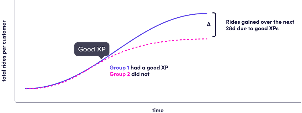
RES is a tool for estimating how various user experiences (low ETA, early driver arrival, etc.) impact long-term rides taken, which is the Δ in Figure 1, without requiring an A/B test.
Challenges in Estimating the Effects of User Experiences
In order to explain RES, I will first discuss the challenges in estimating how user experiences impact rider retention.
The essence of this problem is estimating the causal effect of exposing riders to a particular experience on rider retention. For simplicity, we define the rider retention effect as the impact on the number of rides taken in the future 28 days. The true causal effect of a rider experiencing low ETA would be obtained by observing the future 28 day rides for a rider session in which low ETA is encountered, and comparing that to the future 28 day rides for the exact same rider session, except low ETA is not encountered (counterfactual). But, it’s impossible to observe counterfactuals; in reality, for a given session, we only observe the session where the rider experiences low ETA or not, but not both (the Fundamental Problem of Causal Inference).
A simple potential solution to overcome the challenge of not being able to observe the counterfactual outcome might be to look at historical observational data for riders that experienced low ETA, and compare their average ride retention to riders who didn’t experience low ETA, which is the average treatment effect (ATE) estimated by difference-in-means estimator.
However, this naive approach can lead us astray. Let’s see what happens when we apply this method. Figure 2 shows hypothetical results (not real data) that illustrate the problem we might encounter.

Based on the observations in Figure 2, we would conclude that low ETA actually has a negative effect on rider retention, which must be incorrect. To understand how we arrived at this incorrect conclusion, we segment our data into regions City A and City B, and also indicate on the x-axis whether or not the rider experienced low ETA (left of dashed line didn’t see low ETA, right did); results are shown in Figure 3.
We now see that within City B, and within City A, the effect of low ETA is showing a positive trend, as expected. We also see that City B is much less likely to be in the “treatment” group (right of dash, low ETA), and that City B has higher baseline rides in the next 28 days. We thus see that our groups for low and not low ETA are biased (selection bias), which results in an incorrect estimate of the causal effect of low ETA. The difference-in-means estimator works well for randomized experiments, but is biased for non-randomized cases; in the above example, region is correlated with both the treatment ‘low ETA’, as well as the outcome # of rides in the next 28 days (region is a confounder). This is an example of an issue that can arise when estimating causal effects from observational data.
The gold standard approach for estimating causal effects is randomized experimentation (A/B test). With randomization, we would end up with a roughly equal split of City A and City B across control and treatment groups, thus mitigating the bias discussed above. But, a limitation of an A/B test is that we typically can only run them for a fixed short period of time, which won’t allow measuring long-term effects on rider retention. We thus can benefit from methodology that can mitigate the bias in causal effects estimated from observational data.
RES Methodology
The RES tool employs causal inference methodology to mitigate the bias in causal effects measurements obtained with observational data.
There are various methods to control for confounding variables. Propensity score methods model the relationship between confounders X and treatments W (i.e. with an ML model), outcome methods model the relationship between confounders X and the outcome Y, and double ML methods model both the relationship between X and Y and W and X.
RES employs Augmented Inverse Propensity Score Weighting estimator (AIPW; more info on AIPW can be found here), which is an example of a double ML Method.
At a high level, AIPW consists of estimating potential outcome functions of treatment and control experiences (Direct Method), as well as adjusting estimation bias with propensity weighted residuals. AIPW has the desirable theoretical properties of Neyman Orthogonality (robust to ML estimation errors), and doubly robustness. We also apply a cross-fitting procedure (data split) to get Double-ML properties (unbiased estimation).
More precisely, we compute the treatment effect as follows:

In order to compute the treatment effect, we train three XGBoost or LightGBM models
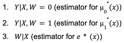
For every observation i, using the above models (and cross-fitting), we predict the outcome μ₁*(xᵢ), μ₀*(xᵢ), and e*(xᵢ). Finally, we plug μ₁*(xᵢ), μ₀*(xᵢ), and e*(xᵢ) into the equation for AIPW to get an estimate for the ATE for low ETA. Though the relationships between outcomes, treatment, and confounders in the above low ETA example are relatively simple, using machine learning models for e*(xᵢ) and μ*(xᵢ) allows us to model complex non-linear relationships which may arise in other settings.
In the example above, AIPW helps us avoid making a wrong conclusion in two ways:
- By modelling the relationship between region and 28-day rides (μ*(xᵢ)), we are able to isolate the effect of region on our outcome Y, and capture that City B riders are more likely to have more rides in 28 days than City A.
- By modelling the relationship between region and low vs. normal ETA (e*(xᵢ)), we capture that City B riders are less likely to experience low ETA than City A riders. AIPW reweights observations inversely to their propensity scores, effectively upweighting points in the bottom-left and top-right of Figure 3. This reweighting reveals the underlying upward slope, allowing us to conclude that low ETA has a positive impact on 28-day rides.
The AIPW estimator combines both 1. and 2., which gives favorable statistical properties, such as treatment effect estimation being insensitive to errors in models e*(xᵢ) and μ*(xᵢ).
What I did as a new hire
The existing RES estimates needed an update, and there was also a need to add additional rider experiences to the RES pipeline. RES generally needed a refresh, and I was tasked with doing so.
I started by gaining more familiarity with AIPW. Reading through the internal causal inference lecture series at Lyft was extremely helpful. I also found Stefan Wager’s STATS 361 course notes very useful for learning about AIPW.
Next, I spent time learning about how to use LyftLearn, Lyft’s internal computing platform for Big Data and Machine Learning. I then became familiar with how to use the RES codebase. I analyzed the RES codebase to see if there were any opportunities to improve reliability and efficiency of the RES code. I identified some aspects of the RES code which could be improved, and then submitted a pull request with the corresponding changes. For example, there was a subtle issue which prevented model diagnostics from completing in certain cases, which I was able to fix.
With the unblocking of the RES pipeline, I sought to compute estimates of long-term effects of various Lyft user experiences. I began with identifying the most important experiences to add to the RES pipeline.
I reached out to other teams to see which experiences would be most important to their work. Examples of experiences that were identified are “Improved Match Time Prediction”, and “Improved ETA Reliability”.
After gathering a list of experiences, I prioritized and selected 23 based on discussions with my manager about their potential impact. This process provided great insight into the experiences that matter most to our riders, and where we could have the greatest positive impact on retention. I also refreshed estimates for the pre-existing reliability experiences (with newly added High Value Mode sub group analysis).
A major challenge I faced in computing estimates for my chosen experiences was selecting confounders. Internal RES documentation provides excellent guidance on selecting confounders, but significant trial and error was still required. For example, I computed RES estimates for Prime Time experience, where Prime Time refers to a multiplier on ride price during high demand periods, and I had included Neighborhood Supply as a confounder. The ROC AUC of our trained model was suspiciously high, which we realized was partly due to Neighborhood Supply being a leaky confounder for Prime Time. A leaky confounder is a covariate which contains information that is concurrent or subsequent to the experience; this is an issue, as it can cause some of the treatment effect to be attributed to the confounder, leading to biased estimates.
For each of the 23 experiences I worked on, I had to make sure to include key confounders, and also avoid including problematic confounders, which was very time consuming. But, this process provided a great opportunity to learn about various data sources that exist at Lyft, and to reflect on how key covariates may be related causally to Lyft rider experiences.
Conclusion
Though I faced many challenges in my starter project, I had excellent support from my colleagues at Lyft, and was able to successfully generate causal estimates for the 23 user experiences identified.
Navigating the various challenges I encountered was a very intellectually stimulating and fulfilling experience. The insights from RES play a crucial role in helping teams focus on the experiences that matter most to our riders; contributing to a workstream with such a high impact on improving rider experience has been very rewarding.
Getting started at Lyft has been an enriching journey. I’ve had the opportunity to apply real-world causal inference techniques and collaborate with amazing colleagues. I’m excited to continue contributing to impactful projects, and to see what the future holds.
Lyft is hiring! If you’re passionate about Data Science, visit Lyft Careers to see our openings.
My Starter Project on the Lyft Rider Data Science Team was originally published in Lyft Engineering on Medium, where people are continuing the conversation by highlighting and responding to this story.


